
‘Can we find outperformance using an algorithmic asset selection approach which focuses on lesser used risk and return statistics?’
Throughout the asset management industry, we observe that fund analysts prefer more ‘traditional’ statistics of their fund/manager assessment – i.e. which fund has a higher Sharpe Ratio?
This post will compare two baskets, created using different statistical indicators and the same algorithmic asset selection methodology, to ascertain if it is possible to achieve outperformance whilst maintaining desirable portfolio characteristics. We will back test these baskets across two hedge fund strategies CTA/Managed Futures and Long/Short Equity.
To create the two baskets data from Eurekahedge was filtered by the following criteria:
| Basket 1 | Weighting | Basket 2 |
|---|---|---|
| Annual Sharpe Ratio (Rf = 0.25%) | 40% | Calmar Ratio |
| Annualised Return | 20% | Rachev Ratio |
| Annualised Volatility | 15% | MVaR 99% |
| Normal VaR 99% | 15% | Annual Up-Capture vs. S&P 500 TR |
| Max Drawdown | 10% | Annual Down-Capture vs. S&P 500 TR |
Table 1 shows our basket statistics and respective weightings. We used the AlternativeSoft ranked search algorithm to find the top six hedge funds under the specific basket criteria and ranking. The statistics selected in basket 1 represent a cross-section of ‘commonly used’ statistics in fund selection. So, why have we selected the criteria in basket 2?
Calmar Ratio1 is an improved version of the Sharpe and Sterling ratios. We have selected this statistic to maximise our returns whilst simultaneously minimising drawdown. Rachev Ratio is a risk reward ratio which measures expected tail gain with respect to expected tail loss. By adding this ratio to the criteria, we are assessing funds based on the potential reward from the right tail with respect to the potential loss from the left tail. Plainly, we are maximising expected tail gain.
Modified Value at Risk, MVaR2, is similar to normal VaR but assumes that our return profile does not have a normal distribution by factoring in both skewness and kurtosis. MVaR will allow us to account for volatility, skewness, and excess kurtosis to choose a basket with the lowest possibility of losing more than the MVaR at the 99% confidence level.
Up/Down Capture allows us to see how the fund will behave relative to our Benchmark, S&P 500 TR, adding this ratio to our criteria will allow us to identify funds which outperform the benchmark under different market conditions. These criteria are important as we wish to see our portfolio have constantly higher returns than the S&P500 TR Index when the markets are doing well and show outperformance when markets are in a downturn.
Two baskets with the top six funds were created for our two respective strategies, based on the criteria in table 1.
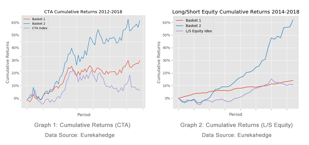
It can be seen from graph 1 that this selection method has achieved 14% outperformance against basket 1, whereas graph 2 shows an even larger outperformance of 48% for Long/Short Equity strategy. It is apparent from both charts that the volatility has increased along with the increase in returns, but have we captured sufficient upside when compared to the benchmark (S&P 500)?
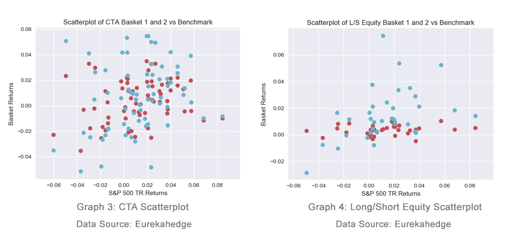
Graph 3 shows the scatterplot of basket 1 (red) and basket 2 (blue) vs. the S&P 500 TR Index. The plot shows our increased volatility but shows there is significant upside being captured compared to basket 1. Graph 4 shows the same scatterplot for the Long/Short Equity baskets, it also shows basket 2 outperformance when compared to basket 1.
| Correlation to S&P 500 TR | Annualised Return | Max Drawdown | ||||
|---|---|---|---|---|---|---|
| CTA | L/S Equity | CTA | L/S Equity | CTA | L/S Equity | |
| Basket 1 | 0.12 | 0.11 | 1.91% | 4.35% | -5.12% | -0.48% |
| Basket 2 | 0.14 | 0.52 | 5.54% | 16.94% | -6.36% | -3.64% |
| Increase/Decrease | 0.02 | 0.41 | 3.63% | 12.59% | -1.24% | -3.16% |
| Eurekahedge Indices | 0.25 | 0.85 | 0.49% | 4.88% | -5.03% | -6.25% |
Data Source: Eurekahedge
Table 2 shows how our choice in asset selection criteria affects the statistics of the equally weighted baskets across both strategies. We can see that we have made a trade-off by increasing correlation and drawdown in pursuit of returns. There is a 1.24% and 3.16% increase in max drawdown as well as an increase in annualised returns of 3.63% and 12.59% for CTA and Long/Short Equity strategies respectively. The Long/Short Equity basket 2 shows a higher correlation to the S&P 500 TR Index which is acceptable as it is below the correlation for the Long/Short Equity Index.
In conclusion, it is possible to achieve higher absolute returns by using the basket 2 criteria stated in table 1. Although these appear to not be well risk-adjusted, the presence of a left tail in basket 2 returns data is from the use of the Rachev Ratio and the expected total loss / expected tail gain trade-off. In practice, one would combine these advanced and traditional approached and use re-sampling / back testing to identify the optimal weight profiles for fund allocation.
It is worth noting that these results are one example and, while the metrics haven’t been back-fitted to game historic data, they perform very well for these time-series across the period of available active returns. A natural next-step for this post would be to optimise the weightings to see if we can achieve better risk-adjusted returns.

71 Carter Lane, London,
EC4V 5EQ
+44 20 7510 2003